Every claim we make about a metal, we can show you the data for.
Mox Core operates its own assay laboratory in Miami, with additional laboratory presence in Nevada, rather than outsourcing verification to a third party. What follows is a real look at how we characterize material on our own bench.
Four methods, one lab.
Depending on the metal, grade, and level of detail a client needs, Mox Core runs one or more of the following in-house testing methods before material ever trades.
Fire Assay
The industry-standard gravimetric method for precious metals, used to determine gold, silver, and PGM content with the accuracy commercial trading and refining require.
XRF (X-Ray Fluorescence)
Fast, non-destructive elemental screening used to identify composition and flag alloy or contamination issues before deeper testing.
ICP (Inductively Coupled Plasma)
High-sensitivity elemental analysis capable of quantifying trace-level concentrations across precious, PGM, REM, and base-metal samples.
OES (Optical Emission Spectrometry)
Rapid metal and alloy composition verification, commonly used for grading scrap, confirming alloy specification, and quality-control checks.
Nanoparticle Tracking Analysis (NTA)
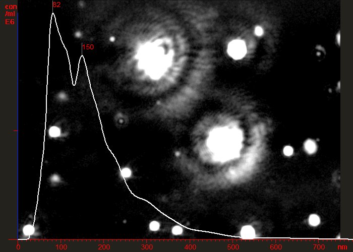
Particle size and concentration are verified using Nanoparticle Tracking Analysis, a laser-illumination technique that visualizes individual nanoparticles in suspension and tracks their Brownian motion on a particle-by-particle basis.
Random particle motion is tracked on video; the diffusion coefficient is calculated and converted to hydrodynamic diameter via the Stokes–Einstein equation, giving us a measured — not estimated — particle-size distribution.
From sample to measurement
Sample preparation
The sample is dispersed in 30% benzyl alcohol (in ethanol) and probe-sonicated for approximately 10 minutes to reduce agglomeration.
Filtration
A 0.2 µm PTFE syringe filter is used on a parallel aliquot to isolate the sub-micron population from larger agglomerates.
Acquisition
120-second video captures per sample, with viscosity normalized to 2.17 cP at 23°C for all measurements, then converted via the Stokes–Einstein relation.
What the data looks like in practice
The charts below are drawn from an actual characterization run on a copper nanopowder sample — unfiltered material compared against a 0.2 µm-filtered aliquot.
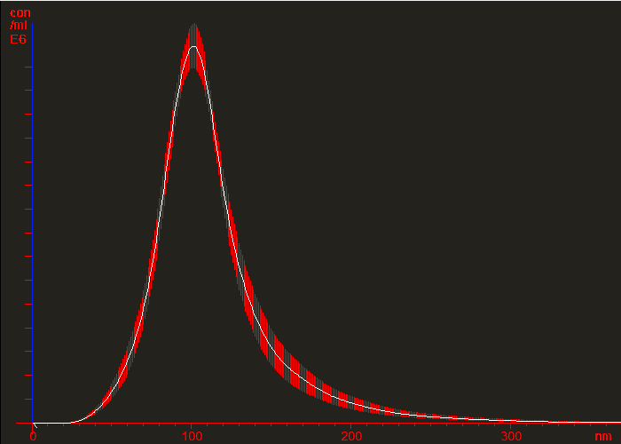
Merged size-distribution profile across replicate analyses — dominant population centred near 100 nm.
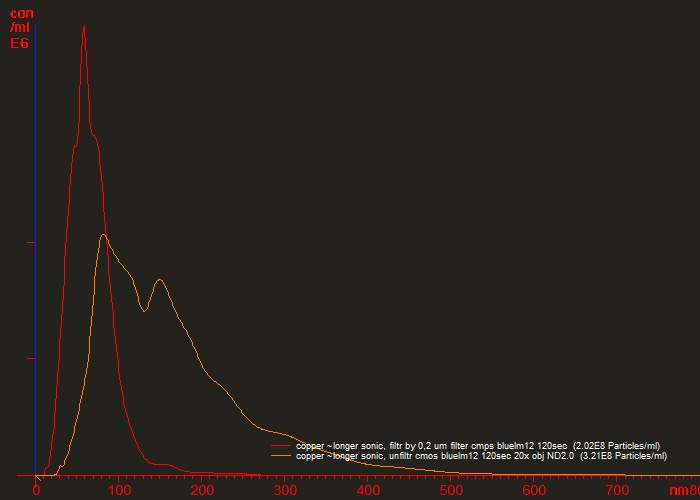
Unfiltered vs. 0.2 µm-filtered aliquot — filtration removes the coarse tail and sharpens the sub-100 nm population.
| Condition | Size range | Modal size | Concentration | Pre-treatment |
|---|---|---|---|---|
| Unfiltered (top aliquot) | ~20–700 nm | 82 + 150 nm | 3 × 10&sup8; particles/mL | Dilution + probe sonication |
| Filtered, 0.2 µm (top aliquot) | ~10–300 nm | 59 nm | 2 × 10&sup8; particles/mL | Dilution + sonication + filtration |
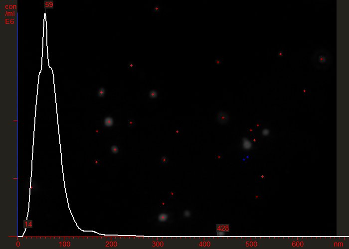
We can show you the particles, not just the chart.
Individual nanoparticles are imaged by laser-illuminated darkfield microscopy prior to trajectory tracking, with each viewing window approximately 100 × 80 µm.
Because NTA cannot count particles above roughly 1 µm, we report the tracked sub-micron population alongside the bulk powder characteristics — not in place of them — so clients see exactly what was and wasn't measured.
What we tell clients, including the caveats
Repeatability
A defined dispersion protocol is applied to every batch to improve run-to-run repeatability of particle-size reporting.
Handling limits
Extended sonication beyond ~10 minutes risks sample overheating; a cooled bath system is used for longer dispersion cycles.
Reporting boundaries
Coarse agglomerates exceeding 1 µm fall outside NTA's tracked range and are disclosed separately rather than folded into the nano-scale figures.
Want to see a certificate of analysis?
Independent NTA characterization data and a certificate of analysis are available on request for any lot.